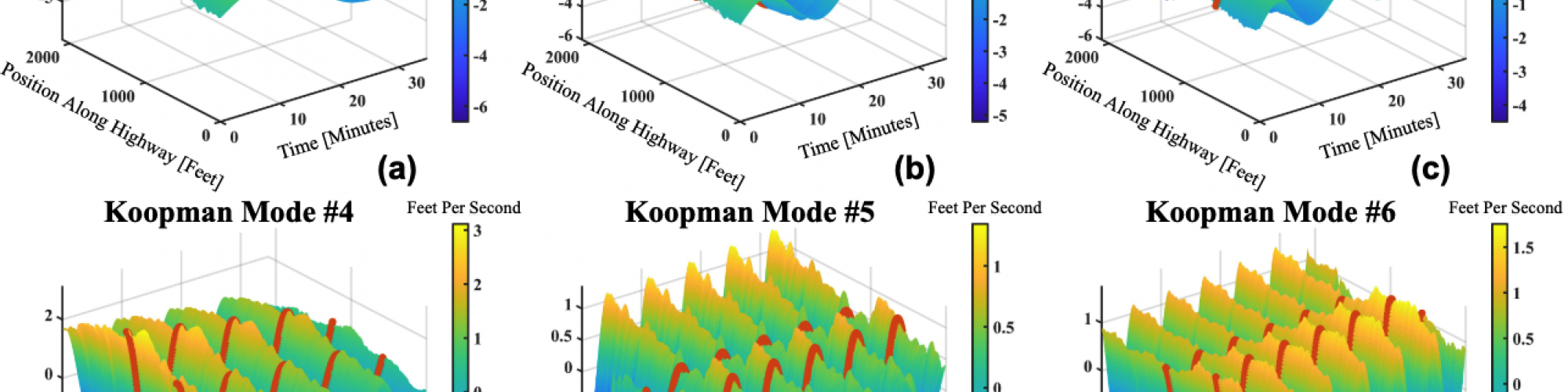
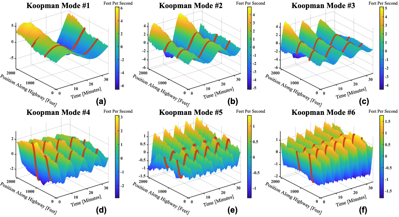
The on/off-ramp locations have been labeled with dark orange dotted lines. Modes one to three have a very localized structure near the post-off-ramp section, indicating that they correspond to pinned localized clusters (PLC). Furthermore, it is evident that the first three modes capture the general transition from high to low velocities that occurs during the onset of traffic. Mode 5 seems to be a spatial harmonic of the first three modes in that it has another peaked structure in the mid-ramp section of the highway. Modes four, and six provide clear evidence for the pumping effect, where an apparent increase in amplitude followed by a decrease can be seen in these modes as they propagate past the off and on-ramps respectively. Overall, the Koopman modes uncover complex spatiotemporal wave structures that are hidden within traffic data. Furthermore, every mode oscillates with a single known frequency, according to the imaginary part of its corresponding eigenvalue. This can be contrasted to a Fourier analysis which would yield modes and frequencies specific to the positions along the highway.

(a-b) Raw data collected from PeMs for the I-10E and southern California network. The data was collected for a week and five days respectively. The I-10 highway seems to be mostly congested throughout the week until Sunday. As expected, all highways within the network seem to be congested on the days leading up to Christmas eve (12/21-12/22). Interestingly, there appears to be drastic relief in congestion during and after the actual holiday dates of 12/24-12/26. (c-d) Forecasted data generated by the MH-HDMD utilizing the last fifteen minutes of data to forecast the next fifteen minutes. The network was forecasted by concatenating data obtained for individual highways and applying the MH-HDMD algorithm to the concatenated data. By visual inspection alone the raw and forecasted data sets are indistinguishable, indicating an accurate forecast.

(a) Map of the multi-lane network obtained from Map data (copyright 2019 Google). The highways studied are highlighted and data for three lanes of both north-south and east-west directions are collected for the entire day of December 20th, 2018. (b) The twenty-four-hour Koopman mode revealing the order of congestion within the network. Specifically, by observing the staggering of the amplitude one can see that during the morning rush the westbound I-105 and I-10 along with the northbound I-405 and I-110 jam first. In the afternoon traffic switches directions and it is the eastbound and southbound directions of the previously mentioned highways which are jammed. This corresponds with the well-known fact the morning commuters generally travel from San Bernardino (east to west) and Orange County (southeast to northwest) into Los Angeles. (\c) A plot of the average phase of the mode sorted by highway confirming the previously mentioned synchrony of congestion. Specifically, the north and west directions seem to be in phase with each other and likewise for the south and east directions. (d) The magnitude of the twenty-four-hour mode along with magenta-colored lines used to visually divide the differing highways. The magnitude of the mode reveals that the eastbound I-10 and I-105 highways are more occupied than the other highways.
The mode has a period of approximately six minutes and the time for each figure is given in minutes-seconds. Mode seven clearly captures the dynamics of a highway wide traffic jam. It is interesting to note how the moving localized cluster's (MLC) travel can be out of phase across differing lanes. This results in the apparent top-left to a bottom-right direction of travel and is a feature impossible to recover from a single-lane analysis. Lastly, one can observe that the on-ramp density of vehicles is not merging at the time of peak congestion. Specifically, the on-ramp is most heavily congested during figures c-d at which point the MLC has already propagated by. However, mode fourteen, a harmonic of this mode, clearly displays the opposite effect. This demonstrates how our multi-lane analysis can be utilized to verify the successful timing of static ramp metering algorithms and identify the correct timescales for dynamic ramp metering algorithms.
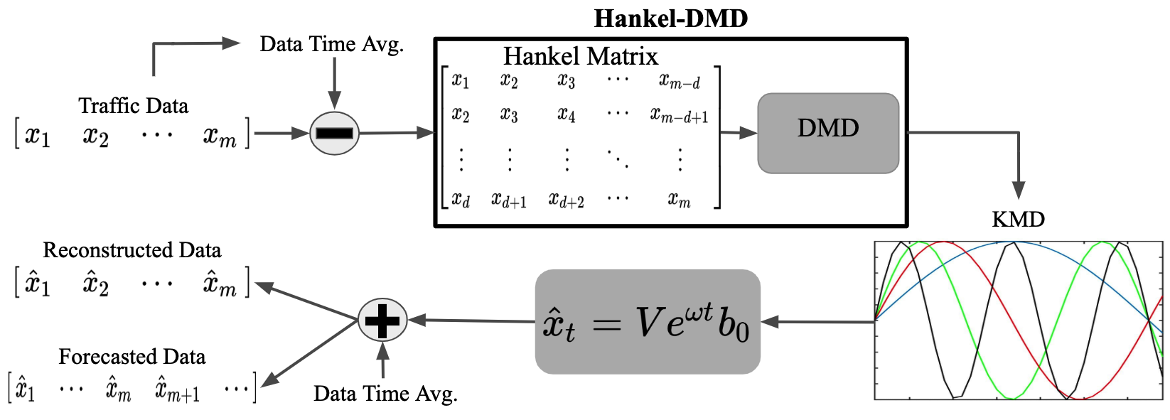
First, the time average of the traffic data matrix is removed. Then the spectral quantities (eigenvalues, modes) of the Koopman operator associated with the mean subtracted data are computed via the Hankel-DMD algorithm. Hankel-DMD consists of applying an exact DMD algorithm to a time-delay embedded data matrix (Hankel matrix). The dimension of the embedded Hankel matrix is now d*n by m-d, where dis the number of delays and n is the size of a single data vector x. Hence a taller data matrix (more rows) is obtained, at the expense of losing d columns. The modes of the Koopman operator can then be evolved via the linear equation they satisfy and superimposed with the previously removed time averages to obtain a reconstruction of the original traffic data or produce forecasts.